Overview
Cancer classification is one of the vital areas of medical sciences. In this project, we examine the Gene Expression data for various types of cancer and classify each cancer into its subtypes. We gather the samples from GEO datasets and select the best features using the class-overlap score, standard deviation by mean ratio, ANOVA – F value and $\chi^2$ (Chi-square) statistics. We then run the following classifiers: K Nearest Neighbors, Naïve Bayes and Decision Trees. We then checked the accuracy of a classifier against a feature selection method for all combinations and observe a feature selection – classifier pair that gives a better accuracy for a particular dataset.
Background
Early discovery of cancer is an important step in determining the treatment of a patient. Gene expression data can be used to predict the presence of cancer. Traditional way of cancer classification uses the physical attributes and the symptoms of the patient to gain a deeper understanding of the patient’s condition. Because causation and spread of cancer is more related to the genes, it is equally important to study the gene expression data.
Goal
Our goal was to use Gene Expression Omnibus (GEO) datasets to build models that can predict the presence of cancer and identify the severity of the cancer. These datasets are freely and publicly available from the NCBI. Each dataset has the gene expression data for various samples, with rows of a matrix file denoting the probe id and the columns denoting the samples. We took five GEO datasets, which have been briefly explained below :
GSE19804 (Lung Cancer Dataset):
GSE19804 is a lung cancer dataset having 120 samples, with 60 lung cancer tissue samples and 60 normal tissue samples, with 54, 675 probe sets.
GSE27562 (Breast Cancer Dataset):
GSE27562 is a breast cancer dataset having 31 normal samples, 57 malignant breast cancer samples, and 37 benign breast cancer samples, with 54, 675 probe sets. There are 15 gastrointestinal tumor and and 7 brain tumor samples, which we have excluded from the datasets as a part of the experiments. We have also excluded 15 breast cancer samples following surgery, since there is no information about them having shown any signs of cancer after surgery.
GSE32474 (NCI60 Dataset):
GSE32474 dataset contains 9 types of different tumors. It has 18 samples for leukemia, 15 samples for breast cancer, 21 samples for ovarian cancer, 21 samples for colon cancer, 26 samples for melanoma, 18 samples for central nervous system, 23 samples for renal cancer and 26 samples for non-small lung cancer, with 54, 675 probe sets. We have excluded 6 prostate samples, since it is not enough for classification.
GSE33315 (Leukemia Dataset):
GSE33315 dataset contains 7 types of leukemia cancer. It has 115 samples of type hyperdiploid, 40 samples of TCF3-PBX1, 99 samples of ETV_RUNX1, 30 samples of MLL, 23 samples of PH , 23 samples of hypodiploid and 83 samples of T-ALL, with 22,283 probe sets. We have excluded 4 CD34 and 4 CD10CD19 samples, since that is too less for classification. We have also excluded 153 samples having no known karyotype to focus on leukemia.
GSE59856 (Pancreatic and Biliary Tract Cancer):
GSE59856 dataset contains 100 pancreatic cancer samples, 98 biliary tract samples, 50 colon cancer samples, 50 stomach cancer samples, 50 esophagus cancer samples, 52 liver cancer samples, 150 healthy samples, with 2555 probe sets.
Challenges
There were two major challenges in this project:
- High number of features
- Low number of samples
These two challenges go side-by-side in this scenario. Probe ids of a series metrix file essentialy denote the genes whose expression value has been recorded. As such, they are the features of the datasets. As an extreme example, the Lung Cancer Dataset (GSE19804) had 54,675 probe ids, while there were only 120 samples in this dataset. This is a very low number of observations as compared to the number of features; a ratio of less than 0.002. Similar is the case for the Breast Cancer Dataset (GSE27562). Other datasets, though not as extreme, suffer from a similar problem of higher number of features as compared to the number fo observations.
Actions
In order to get rid of the curse of dimensionality, we tried variety of methods for feature selection and model, depending on the data. A simple example of this the Lung Cancer Dataset (GSE19804). A plot of the features with high variance in this dataset looked like this:
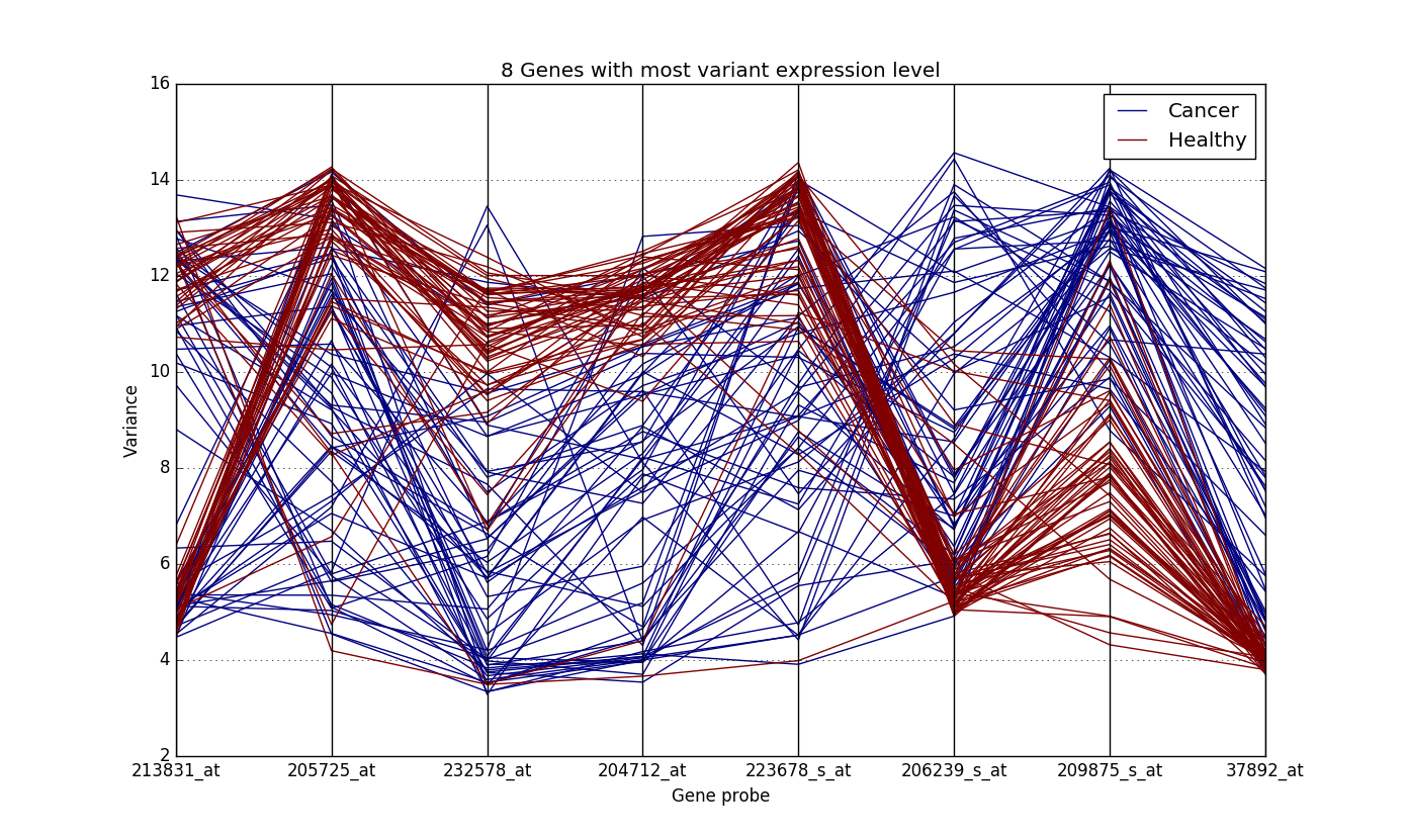
The y-axis denotes the expression values of the genes. It is quite clear from the plot how the expression values of genes are different for the healthy samples and the ones with cancer. While the expression values of genes of cancer patient are all over the place, those of the healthy sample are concentrated at particular locations.
This distinction is more clear in the radial visualization of these 8 genes:
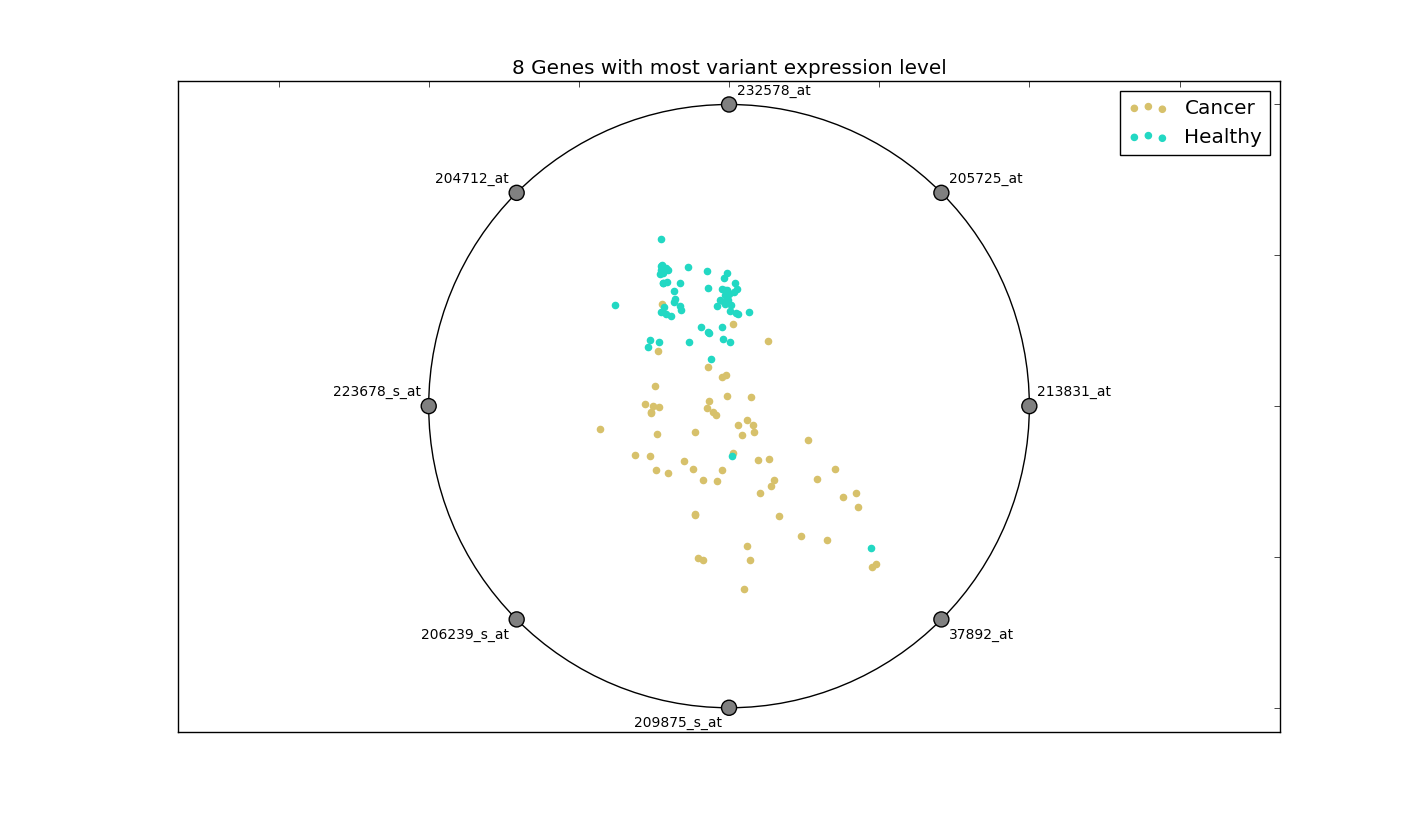
This plot displays relative expression values of the 8 genes. The higher the normalized value of expression, the closer the observation is to the gene. It can be seen how the genes of a healthy person form a cluster, while those of a cancer patient are spread over. As such, simply selecting the features with high variance may work in this case.
This method doesn’t work in other cases though. Take an example of the NCI60 Dataset (GSE32474):
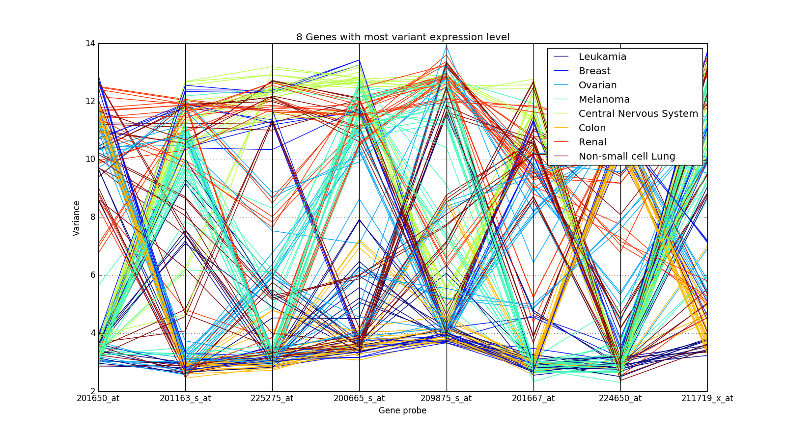
The expression values of the genes are crossing over for different cancer types and hence it is not easy to distinguish them.
Because of different distributions of the datasets, we tried different methods for feature selection. These methods were class-overlap score, standard deviation by mean ratio, ANOVA – F value and $\chi^2$ (Chi-square) statistics. Additionally, we tried different machine learning models, including KNN, Naive Bayes and Decision Trees. These were combined with the feature selection methods to get the best results, making the selection by trial and error.
Results
We ran our experiments using stratified random sub-sampling validation. The stratified approach was taken to avoid the effects of unbalanced classes in the datasets. Random sub-sampling was done, instead of k-fold cross validation, since the number of samples in the datasets are quite low. These validations were repeated 10 times for each combination, and the average results were noted. F1 score was used as the metric to measure the performance.
The results for the five datasets can be seen below.


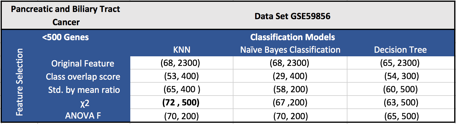
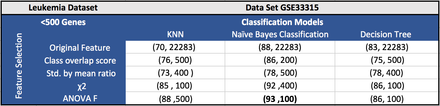
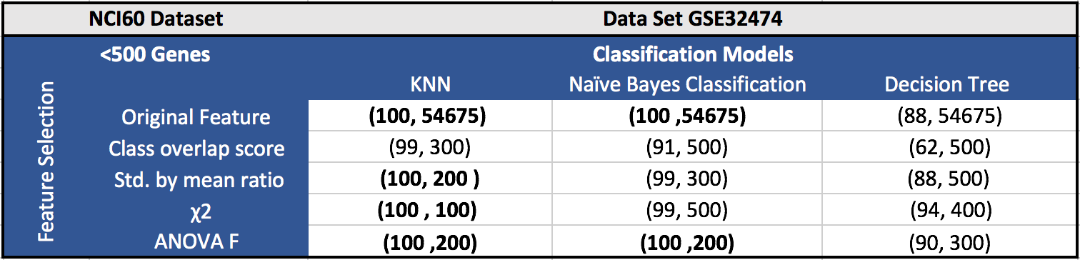
Each cell in a table has (F1 score, number of features). Around 100 features gave the best results in most of the cases.
Further scope
Complete report of the project can be seen here