What is the need to look beyond p-value?
In my last post, I mentioned how we can use p-values to select important variables in a linear model. In general, this sounds like an easy basis of testing a hypothesis, but that is not where the story ends.
In a practical setting, you need to look beyond mere p-value of an experiment. To understand why, let us walk through an example. We will generate our own dataset for this example.
library(dplyr)
library(lattice) # for splom
library(ggplot2)
# Correlation matrix
M = matrix(c(1, 0.7, 0.7, 0.4,
0.7, 1, 0.25, 0.3,
0.7, 0.25, 1, 0.3,
0.4, 0.3, 0.3, 1), nrow=4, ncol=4)
# Cholesky decomposition
L = chol(M)
nvars = dim(L)[1]
set.seed(1)
# number of observations to simulate
nobs = 1000
# Random variables that follow an M correlation matrix
r = t(L) %*% matrix(rnorm(nvars*nobs, mean = 50000, sd = 5000), nrow=nvars,
ncol=nobs)
salesdata = t(r) %>%
as.data.frame()
names(salesdata) = c('sales', 'tv', 'socialMedia', 'radio')
# Plotting and basic stats
splom(salesdata)
summary(salesdata) %>%
knitr::kable()| sales | tv | socialMedia | radio | |
|---|---|---|---|---|
| Min. :33934 | Min. :54906 | Min. :35172 | Min. :52072 | |
| 1st Qu.:46584 | 1st Qu.:66961 | 1st Qu.:46225 | 1st Qu.:65903 | |
| Median :49820 | Median :70901 | Median :49618 | Median :69518 | |
| Mean :49901 | Mean :70639 | Mean :49703 | Mean :69451 | |
| 3rd Qu.:53529 | 3rd Qu.:74194 | 3rd Qu.:53221 | 3rd Qu.:72973 | |
| Max. :65770 | Max. :87670 | Max. :69830 | Max. :84702 |
Now we have a dataset for sales, with 3 independent features: tv, socialMedia, and radio. We have generated 1,000 observations. Each observation consists of data for a particular market. The 3 features give us the amount spent in USDs in different methods of advertising. The sales column has the corresponding sales in that market.
Now that we have the data, let’s build a linear regression model taking all 3 features.
model <- lm(sales~., data = salesdata)
summary(model)
Call:
lm(formula = sales ~ ., data = salesdata)

Residuals:
    Min      1Q  Median      3Q     Max
-7097.0 -1723.0    49.7  1652.5  7543.8

Coefficients:
              Estimate Std. Error t value Pr(>|t|)
(Intercept) -2.124e+04  1.308e+03 -16.242  < 2e-16 ***
tv           5.621e-01  1.552e-02  36.225  < 2e-16 ***
socialMedia  5.348e-01  1.553e-02  34.446  < 2e-16 ***
radio        6.991e-02  1.586e-02   4.409 1.15e-05 ***
---
Signif. codes:  0 '***' 0.001 '**' 0.01 '*' 0.05 '.' 0.1 ' ' 1

Residual standard error: 2389 on 996 degrees of freedom
Multiple R-squared:  0.7888,    Adjusted R-squared:  0.7882
F-statistic:  1240 on 3 and 996 DF,  p-value: < 2.2e-16
All 3 features have a low p-value as per our model. Wonderful! Also, the coefficients of all 3 features are positive. This means investing more in these methods is related to an increase in sales.

Hold on!
Statistical significance means that you can conclude that an effect exists. It is a mathematical definition. It does not know anything about the subject area and what makes up an important effect.
Let’s go back to looking at the coefficient of radio. The low p-value means the effect is significant. Its coefficient is approximately 0.069. This means an extra \(\$10,000\) invested in radio advertising is related to a sale of around 690 more units. The question that arises at this point is this: Is that extra investment worth it?
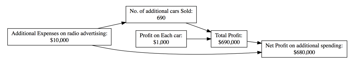
Suppose this data is for a particular car model, for which sale of each car results in a profit of \(\$1,000\). An increase in \(\$10,000\) of spending on radio advertising would be related to a sale of around \(690\) more cars. Sale of \(690\) more cars would mean an extra profit of \(\$690,000\). That is a net profit of \(\$680,000\) on that extra spending. That is \(68\) times the extra money invested in radio advertising.
Consider a different scenario where this data is for the sales of a particular watch. Sale of each watch results in a profit of \(\$10\). An increase in \(\$10,000\) of spending on radio advertising would mean a sale of around \(690\) more watches. Sale of \(690\) more watches would mean an extra profit of \(\$6,900\). That is a net loss of \(\$3,100\) on that extra spending.
How do we check the practical importance of the statistically significant result?
Identify the effect needed for practical importance
A simple solution would be understanding how much effect is important to you. Suppose you were checking if more spending on radio advertising leads to more sales. Additionally, you want to know if spending more on radio advertising leads to at least a net profit of \(5\)X on that extra spending.
As per the model, an increase in spending on radio advertising is related to an increase in the sales.
In the first example, there is a net profit of \(68\)X on the extra investment. As such, statistical significance is of practical importance in this case.
In the second example, spending more on radio advertising is not related to profit. In fact, more spending on radio advertising leads to a net loss of \(0.31\)X times on that extra spending. Thus, in spite of the effect being significant, it is of no practical importance.
Use Confidence Intervals
The coefficient you have is a point estimate of the true coefficient. Since it is an estimate, there is a scope of error. This uncertainty occurs because we have sampled our dataset from some distributions. They do not represent the complete distribution, or in other words, the population. The standard error for that estimated coefficient gives that scope of error. It is the average difference between the estimated coefficient and the true coefficient. For a different dataset with similar distributions, the estimated coefficients may be different.
You can use the standard errors to compute the confidence intervals. A \(95\%\) confidence interval is a range for which we are \(95\%\) confident that it has the true coefficient. In R, we can use the function confint() to find the \(95\%\) confidence interval.
confint(model) 2.5 % 97.5 %
(Intercept) -2.380331e+04 -1.867165e+04
tv 5.316057e-01 5.925002e-01
socialMedia 5.043114e-01 5.652431e-01
radio 3.879204e-02 1.010260e-01The \(95\%\) confidence interval for radio’s coefficient is [0.038, 0.101]. In other words, we can say with \(95\%\) confidence that the true coefficient for radio lies between \(0.038\) and \(0.101\). An increase in \(\$10,000\) spent on radio advertising would mean an average increase in sales from \(380\) to \(1,010\) units.
This is a wide range, but why is that a problem?

Going back to the previous example of cars, the estimated extra profit was \(\$690,000\). As per the confidence interval of [0.038, 0.101], this may range from \(\$380,000\) to \(\$1,010,000\). This means the net profit may range from \(\$370,000\) to \(\$1,000,000\) on the extra spending. In a general sense, the net profit may range from \(37\)X to \(100\)X on any extra spending on radio advertisement in that case. The amount of uncertainty is quite huge. It might be a better idea to invest in a different method instead with less uncertainty.
Conclusion
A p-value is a good starting point to check the importance of an effect. That’s what it is though – a starting point. Once we know of a significant effect, we need to look further into its practical importance.
Sources
- An Introduction to Statistical Learning, with Application in R. By James, G., Witten, D., Hastie, T., Tibshirani, R.
- R Bloggers
- Statistics by Jim
- Stack Exchange
- Stack Overflow
- Slideshare
- Images: Google Images